Speech Emotion Recognition

Context

Emotion detection from speech is a notoriously hard problem. Audio signals are noisy, culturally variable, and existing models struggle with real-world accuracy. Most approaches either oversimplify by treating it as a basic classification task, or reach for compute that makes them impractical to run anywhere near real time.

I built a pipeline that goes the other way: light enough to run in real time, and built on features that encode what the ear actually hears rather than raw waveform samples.

Signal to label

Nothing in that chain is decorative, and the order is the argument. Each stage discards something the next one does not need: the features drop phase and most of the speaker's timbre, the convolutional half drops absolute position, and the recurrent half is the only part that still knows what happened first.

Features over waveforms

Every clip is transformed into a multi-dimensional feature matrix before the model ever sees it: forty mel-frequency cepstral coefficients, twelve chroma bins, spectral contrast, and tonnetz features, all extracted with Librosa. This is the decision the whole project rests on.

A raw waveform is a very long list of pressure samples, and nearly all of that length is detail the task does not care about: phase, the precise shape of one vowel, the room the recording happened in. Emotion lives somewhere else. It lives in how energy is distributed across frequency bands and how that distribution moves across a sentence, which is exactly what these four families of features measure. MFCCs compress the spectral envelope onto a mel scale, which is a model of how human hearing actually resolves pitch, so the representation arrives already weighted toward differences an ear would notice rather than differences a microphone would record. Chroma folds energy onto the twelve pitch classes and picks up intonation, spectral contrast separates the peaks from the valleys in the spectrum, which is close to what a listener hears as tense versus breathy, and tonnetz reads the harmonic relationships underneath.

Hand a convolutional network the raw audio instead and it has to rediscover every one of those properties from examples, and on a dataset this size there are not enough examples to do it. MFCCs and spectral features beat raw waveform input by a significant margin here, because those hand-crafted features encode psychoacoustic properties a CNN has no chance of learning from scratch at this scale. The second half of the argument is cost. A feature matrix is far smaller than the samples it came from, and that reduction is what makes real-time inference possible at all rather than a nice property to have.

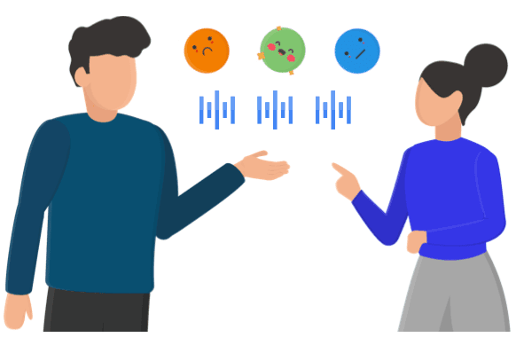
CNN plus LSTM

The classifier is a CNN-LSTM hybrid in TensorFlow and Keras. Convolutional layers read the spatial structure of the spectrogram, the frequency patterns, and LSTM layers capture how those patterns move over time. The temporal half is what separates emotions that share a pitch profile but differ in rhythm, which is most of the interesting confusions: anger and excitement sit in similar registers and are told apart by pacing and attack, not by pitch. Dropout and batch normalisation keep it from memorising a small training set.

Training data is scarce in this domain, so the effective dataset was roughly tripled with noise injection, time stretching, pitch shifting, and random cropping. RAVDESS and TESS were combined so the model saw more than one set of speakers, accents, and recording conditions, which is the cheapest available defence against a model that has quietly learned one studio instead of one emotion.

The problems worth naming

Class imbalance was the first: happy and sad have far more samples than disgust or surprise, handled with SMOTE oversampling and a class-weighted loss. Speaker independence was the second, and the more dangerous one, because a model trained on one speaker will happily score well and then fail on a new voice. A random split hides that failure completely, since the same speaker sits on both sides of it, so speaker-independent cross-validation splits were the only way to know whether it generalised at all.

Latency was the last. The feature extraction pipeline was optimised until a three-second clip processes in under two hundred milliseconds, fast enough that the Flask and React inference interface feels immediate rather than batched. That number is a product constraint rather than a benchmark: past roughly a quarter of a second, a response stops reading as a reaction and starts reading as a computation.

This became the foundation for the IEEE social robotics work that followed.